
Wasteful behaviors predict 47% of provider spending variation
Sometimes little disparities add up to big differences in the bottom line. That’s certainly true when it comes to controlling costs through the stewardship behaviors of healthcare providers, according to our eight-month study with 287 physicians we conducted using data on patient discharges. We examined this key issue among hospital managers and physician group leaders to better understand financial variations within physician inpatient ordering behavior. Through our relationship with over 250 healthcare facilities, we were able to develop a set of provider medication and lab orders that are markers for potential wasteful behavior (for example, repeated daily orders of B-type natriuretic peptide testing). The study indicated that a provider’s propensity to engage in these wasteful behaviors is a strong predictor of that provider being a high-cost outlier, even when controlling for patient acuity (R2 = .467). When providers are gently “nudged” to stop these wasteful behaviors (with a clinical pearl of wisdom and its literature citation), their average spend on medications and labs goes down, and declines by an amount that exceeds the sum of the specific suggestions for cost savings. We hypothesize that reinforcing a “stewardship ethos” causes providers to be more judicious overall, even in areas that fall outside of those presented overtly by IllumiCare. We also show that good stewards order fewer and less expensive tests and medicines, rather than shifting the cost of those orders to other providers on the case.
Research Highlights
An eight-month study of 287 physicians identified as Hospitalist, Internal Medicine, or Family Medicine providers who placed at least 50 orders and cared for at least 15 patients.
The goal was to develop a method to directly measure behaviors that correlate with higher spending and to determine if an effective method exists to intervene on those behaviors in a way that reduces both the behaviors specifically and spending generally.
It was found that when providers are “nudged” to stop wasteful behaviors, their average spend on meds and labs goes down by an amount that exceeds the sum of the specific opportunities identified.
Analysis shows that for every 1 dollar of decrease in average savings opportunities per provider per patient, the clinician actually saves up to 1.5 times that amount per admission.
“Advanced stewards” that embrace financial stewardship opportunities are able to reduce the cost of care while maintaining the quality of care delivered.
A FOCUS ON PROVIDERS
IllumiCare serves hospitals by collecting real-time clinical data about inpatients and wholesale cost data (not charges) on medications and lab tests. The data is used to calculate a real cost of every medication and lab order, attribute that cost to the ordering provider, and aggregate those costs at the patient admission and DRG levels.
This study shifts the focus off patient characteristics and onto physician habits, a change from previous studies that utilized highly advanced models including artificial neural networks, ridge regression models, and other techniques to predict the individual patient’s cost. Those studies used patient demographics such as age, gender, ethnicity, and comorbidities as predictors of individual costs.i
Leep Hunderfund et al. surveyed physicians and medical students, finding that 88% of respondents moderately or strongly agreed that “trying to contain costs is the responsibility of every physician.” ii The AMA Code of Medical Ethics states, “Physicians also have a long-recognized obligation to patients in general to promote public health and access to care. This obligation requires physicians to be prudent stewards of the shared societal resources with which they are entrusted.” iii
Despite calls for provider stewardship, studies show large variation in provider spending on similarly sick patients, even within the same specialty and in the same hospital.iv Higher spending may be an acceptable tradeoff for better outcomes, although it does not correlate with better outcomes.
What is needed is a method to directly measure behaviors that correlate with higher spending and to intervene on those behaviors in a way that reduces both the behaviors specifically and spending generally.v
Materials and Methods
Stewardship Opportunities Considered
Over the past six years, IllumiCare has accumulated a set of medication and lab orders that represent very likely wasteful care (Stewardship Opportunities or “Opportunities”). A medication example is the use of IV Tolvaptan over oral Urea when the patient’s sodium is 128 or above. A laboratory example is repeat daily ordering of B-type natriuretic peptide (BNP) whether or not the test result is normal or abnormal.
A single provider may have responsibility for some of these decisions, such as repeat BNP orders. Other decisions may represent missed opportunities for cost stewardship among multiple providers. For example, switching from IV to PO represents an opportunity where the original IV order was appropriate, but later the patient commenced other PO meds and the PO medication was clinically equivalent. Often, multiple providers failed to make the switch. In this analysis, we included only opportunities that were the responsibility of a single provider. We evaluate the relationship between a provider’s Opportunity per patient (calculated by summing the costs of the wasteful orders of that provider) - the independent variable denoted \({ x }\)- and that provider’s overall medication and laboratory spend per patient - the dependent variable denoted \({ y }\).
Data Collection and Preprocessing
Data on patients discharged between 01 November 2020 to 30 June 2021 was collected through the participating health systems’ HL7 data feeds. Only pharmacy-verified medication orders and resultant laboratory orders were evaluated. Costs for services were attributed at the CMS allowable rate, and cost for medications were attributed at the average wholesale price obtained from Medi-Span. Charge codes were not used in this analysis.
Only orders placed by providers registered with CMS under taxonomy code 208M00000X (Hospitalist), 207R00000X (Internal Medicine), or 207Q00000X (Family Medicine), or who was identified as a Hospitalist, Internal Medicine, or Family Medicine provider by the hospital system under the terms of an IllumiCare SmartRibbon user were included in this analysis. All 284 included providers will be referred to as “hospitalists” in this analysis.
Only orders associated to a patient encounter discharged as “Inpatient” were included. A provider is defined as “caring for” an inpatient encounter if they placed at least 25% of the orders on the discharged patient. Only orders in which the hospitalist was the direct ordering provider, per HL7 order messages, were included in the calculation. So, for example, if a hospitalist instructed a nurse practitioner to place an order, that order was not attributed to the hospitalist.
In sum, this analysis considered 17,032 patient encounters and 30,930 “violating” orders (28,448 lab orders and 2,482 med orders).
Independent Variable
The entire CMS allowable cost of a laboratory order was designated as a cost-saving opportunity. For medication orders, the opportunity was calculated as the difference between the daily unit cost of the ordered medication and the daily unit cost of the lower-cost medication, multiplied by the timestamp interval difference between prescription start and prescription end. This opportunity, for example, is only presented for IV to oral switches when the patient is on another oral medication. A hospitalist’s opportunity per patient is calculated as the sum of all orders that were identified as opportunities divided by their total number of “cared for” inpatient admissions.
Dependent Variable
Hospitalists’ risk-adjusted spend per patient is calculated as \({\frac{1}{n} \sum^n_{i=1} \frac{y_i}{w_i}}\), where n is the distinct number of patients treated, y is the subject hospitalist’s total medication and laboratory spend on the patient, and w is the MS-DRG weight of the patient. In other words, it is the sum of the value of all medication and laboratory orders placed by that provider on a patient that they cared for divided by the assigned MS-DRG weight, divided by the total number of inpatient discharges that they cared for.
Outcome Measures
Because we are evaluating the relationship between the two variables, our outcome measures were focused on directional relationship, variation, and correlation. Our key measures were the Coefficient of Determination (R2), Root Mean Squared Error (RMSE), and Mean Absolute Percentage Error (MAPE). R2 is calculated as \({ \frac{\sum (\hat{y}-\bar{y})^2}{\sum y-\bar{y})^2} }\), or the sum of squares regression divided by the sum of squares total. This value, often expressed as a percentage, gives us the proportion of variability explained in the model among the total variability.vi In our case, how much does a provider’s opportunity per patient explain their overall spend per patient? RMSE is calculated as \({ \sqrt{ \frac{1}{n} \sum^n_{i=1} e^2_i } }\) where \({ e_i }\) is the error of samples \({ i }\). RMSE was chosen because it is more sensitive to variances within the model error than the mean absolute error by penalizing errors with a larger absolute value.vii MAPE is calculated as \({ \frac{1}{n} \sum^n_{i=1} \left| \frac{\hat{y}_i - y_i}{y_i} \right| }\), meaning the average absolute percentage error a predicted point was from the true value, across the data. MAPE is utilized for its intuitive interpretation on the quality of a regression model, its handling of relative variation instead of absolute variation, and its ability to handle both positive and negative errors within our model.viii
Statistical Analysis and Dataset Preparation
The relationship between a hospitalist’s spend per patient and opportunity per patient was assessed through an ordinary least squares (OLS) regression, residuals analysis using diagnostic plots, train-test validation of the model, and comparison of time series.
In the first dataset used for the OLS regression model, the unit of analysis was an individual hospitalist. To prepare the dataset, a hospitalist’s independent and dependent variables were calculated using data over the entire evaluated timespan. For a provider to be included in this dataset, they must have placed at least 50 orders and cared for at least 15 patients. Using random assignment, the hospitalist data was split into a training set (80%) and test set (20%). The training set included 215 hospitalists and the test set included 54 hospitalists. The independent variable x was right skewed, causing the model to be heteroskedastic. OLS regression assumes \({ V(e_i) = \sigma^2 }\) for all values i, meaning the error terms have a constant variance (homoskedasticity).ix A logarithmic transformation was performed on the independent variable using \({ log_e(x+1) }\) to account for this. By adding the constant of 1, we were able to apply the logarithmic transformation to values \({ x=0 }\).
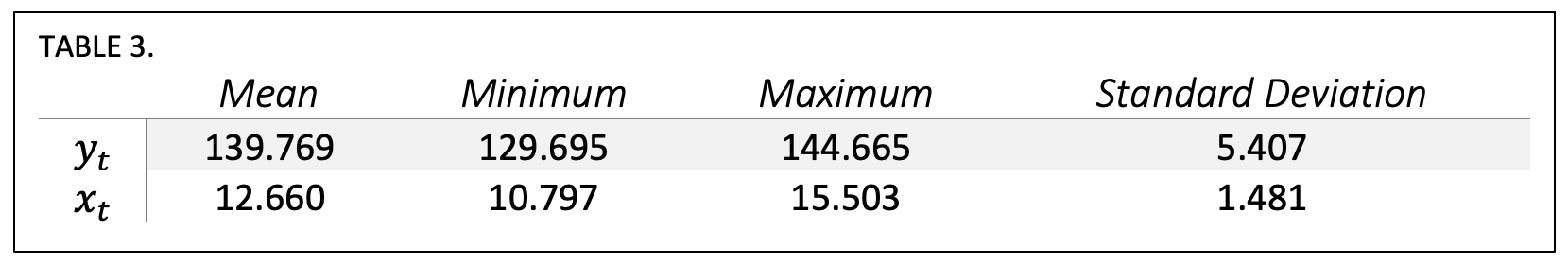
In the second dataset used for time series analysis, the unit of analysis was the mean value among hospitalists per month, i.e., the mean hospitalist opportunity per patient each month or the mean hospitalist spend per patient each month. Costs were attributed to the month in which a patient was discharged. A hospitalist’s independent and dependent variables were calculated as the sum cost for that month, divided by the number of patients cared for and discharged during that month. The mean value per month was calculated to achieve the monthly rate for each variable. A provider must have cared for at least five patients per month to be included.
Results
Descriptive Statistics
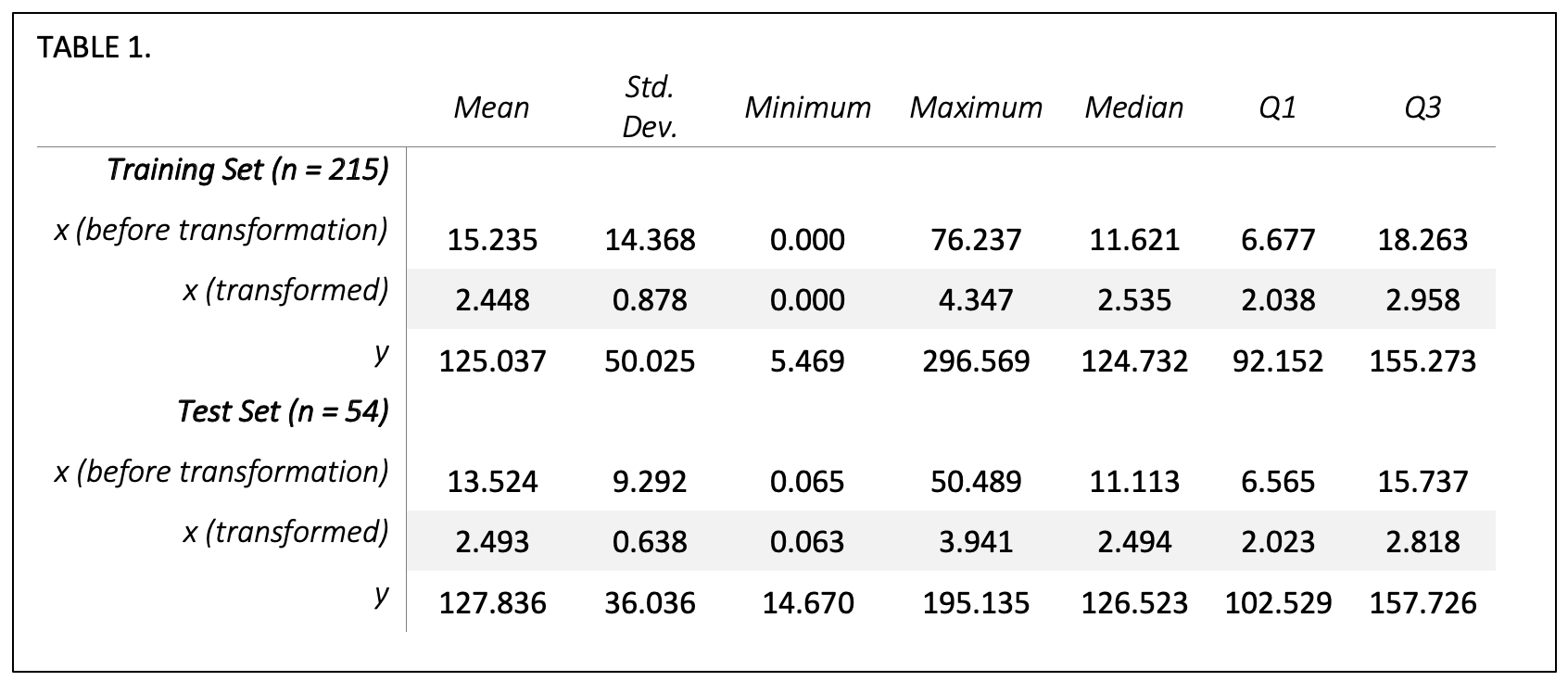
Table 1 describes the distribution of our dependent and independent variables. Opportunity per patient, x, is summarized in the table both before and after transformation, so that the distribution of hospitalists’ opportunity can be evaluated both in real dollar terms and in the log-transformed terms used in our regression model. A two-sample t-test of the training set and test set dependent variables resulted in a p-value=0.699 and of the transformed independent variables resulted in a p-value=0.724, indicating that there are no significant differences in the means of the two datasets.
Ordinary Least Squares (OLS) Linear Regression
In Figure 1 we use the training set to depict the relationship between each provider’s (n=215) independent and dependent variables, with a marginal histogram to visualize the distribution. Each point represents a hospitalist, and the blue line indicates the line of best fit. The training model resulted in a R2 = 0.458, with a p-value < 0.001 and residual standard error of 36.9 on 213 degrees of freedom. 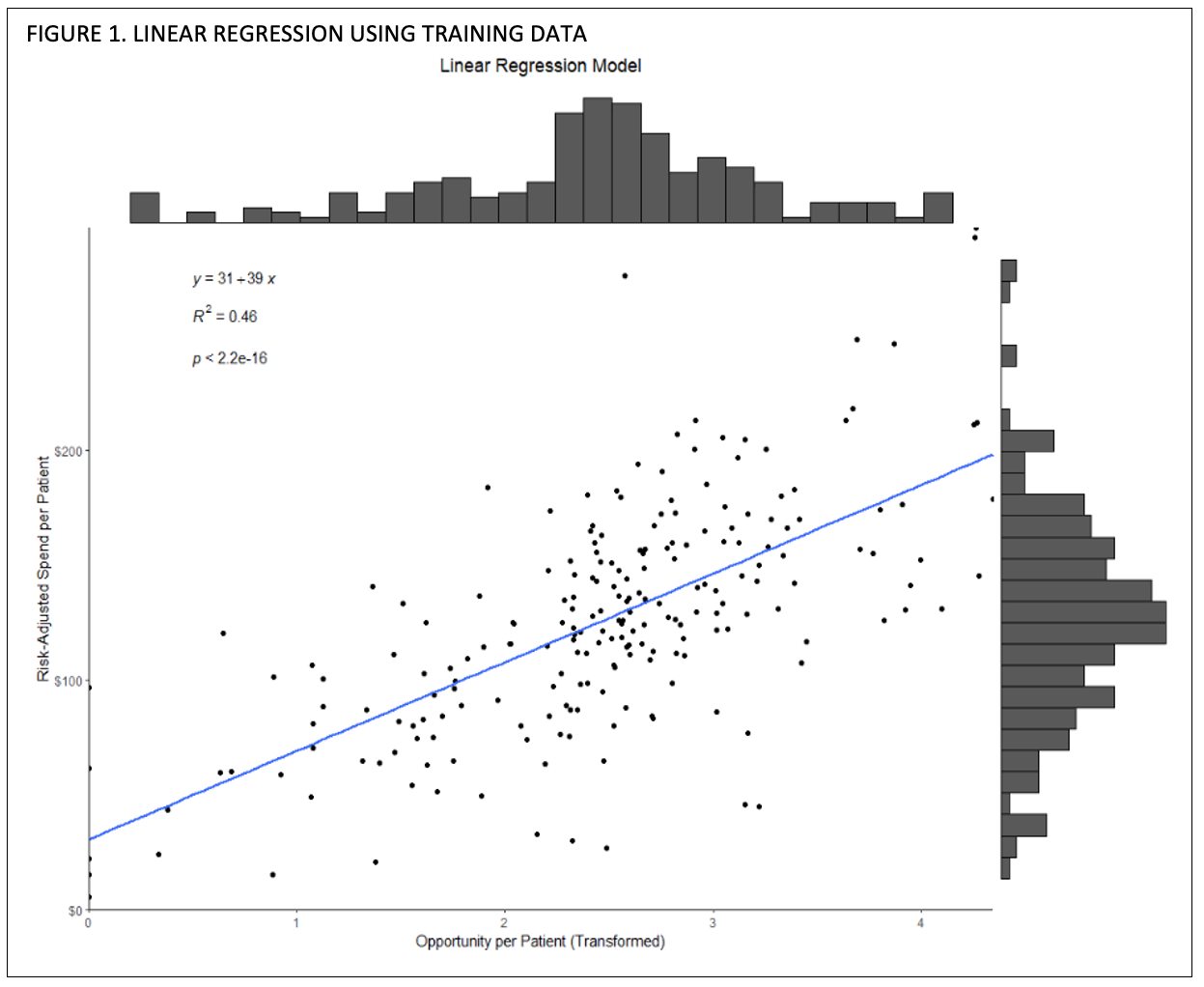
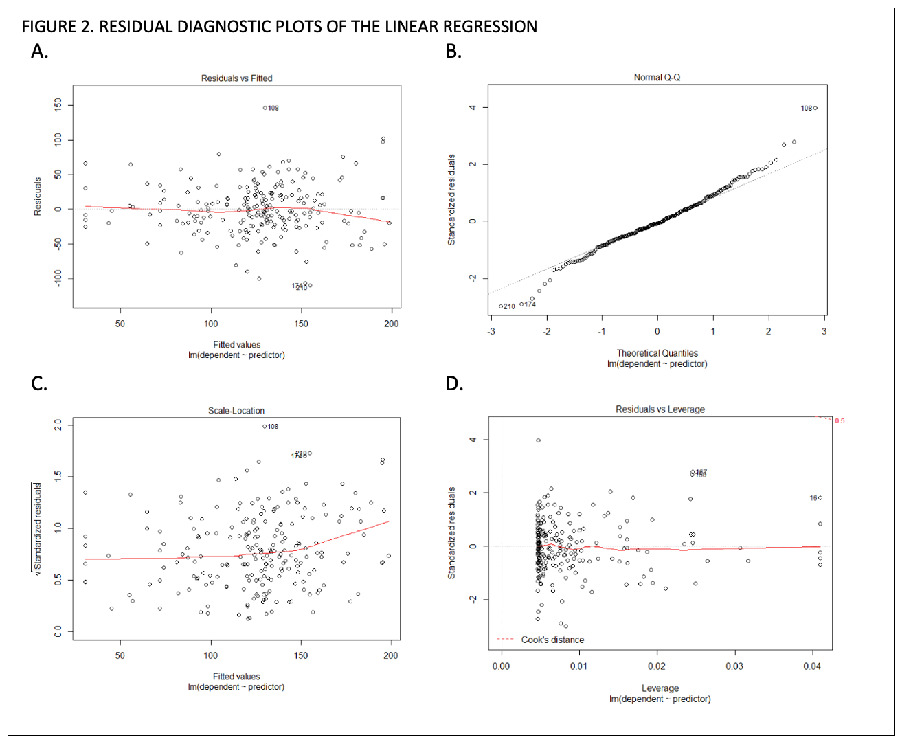
While the distribution looks linear, we analyze the residual diagnostic plots in Figure 2 using R’s plot() function with defaults.
Figure 2A displays the residuals vs fitted values, where the residual on the y-axis is calculated as \({ r_i = y_i+\hat{y}_i }\), or the observed y value minus the predicted value, and the x-axis is the fitted (predicted) value \({ \hat{y}_i }\). If residuals do not show a trend and are spread randomly, then that is a good indication that our variables share a linear relationship and there is not an underlying non-linear trend, such as an exponential increase. x
Figure 2B and 2C, the normal quantile-quantile (normal q-q) plot and scale-location plot, evaluate normality and homoskedasticity of the residuals. Values in the normal q-q plot in 2B generally follow the 45-degree reference line so we can assume normality. The scale-location plot is similar to the residuals vs fitted plot in that it is ideal to see a random spread, though the scale-location plot is used to evaluate the variance in errors to detect heteroskedasticity.xi We see in Figure 2C that our errors do not show a trend, so we fulfil the assumption that our dataset is homoscedastic and errors εi have a constant variance.
Figure 2D, residuals vs leverage, is used to detect outliers and determine whether any point (a provider) significantly affects the model.xii A point with a large Cook’s distance doesn’t fit well with the model and trend, and can greatly affect the slope and R2.xiii Because we do not have any points past the Cook’s distance line, we can infer that no hospitalist included in our dataset is an outlier or significantly goes against the trend.
With our model trained, we calculated RMSE and MAPE to measure the goodness of our model. When running our training data back through the model, the RMSE = 36.728 and the MAPE = 33.1%. When feeding new data into our model using the test dataset (n = 55), RMSE = 24.363 and MAPE = 18.7%, meaning our model’s accuracy was slightly better when evaluating new hospitalists’ data. The original dataset before random assignment was run and resulted in R2 = 0.467.
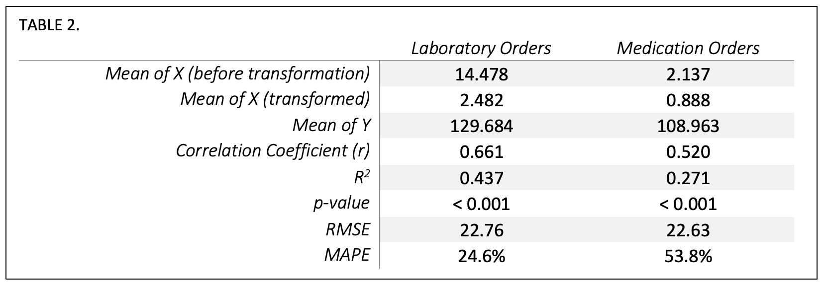
Subcategory Analysis
With our model validated, we reran the analysis in three ways. We evaluated all med/lab cost data (the dataset before randomly splitting into train/test sets), laboratory-only cost data, and medication-only cost data. We can see that the laboratory-only (R2 = .437) or medication-only (R2 = .271) models do not explain variability as well as the combined order spend (R2 = .467) although their variables are still highly correlated and their p-value shows a highly significant relationship.
Monthly Time Series Analysis
We observed an overall relationship in the linear model between provider spend per patient and provider opportunity per patient, so we then wanted to evaluate whether over time there was a directional relationship between opportunity and spend. Our previous independent and dependent variables were then evaluated as timeseries xt and yt respectively.
Monthly characteristics
Time Series Relationship
Figure 3 visualizes the time series with a regression trend line, with yt appearing on top and xt appearing on bottom. The regression slope β1 of yt is -0.251 and the slope β1 of xt is -0.303, meaning for every $1.00 opportunity reduction per provider per patient, there was a $0.82 decrease in average risk-adjusted hospitalist spend per patient. Using the average monthly case mix index of 1.88 of the included patients, we can extrapolate that this is a change of $1.54 in real dollars per patient for each dollar in opportunity reduced.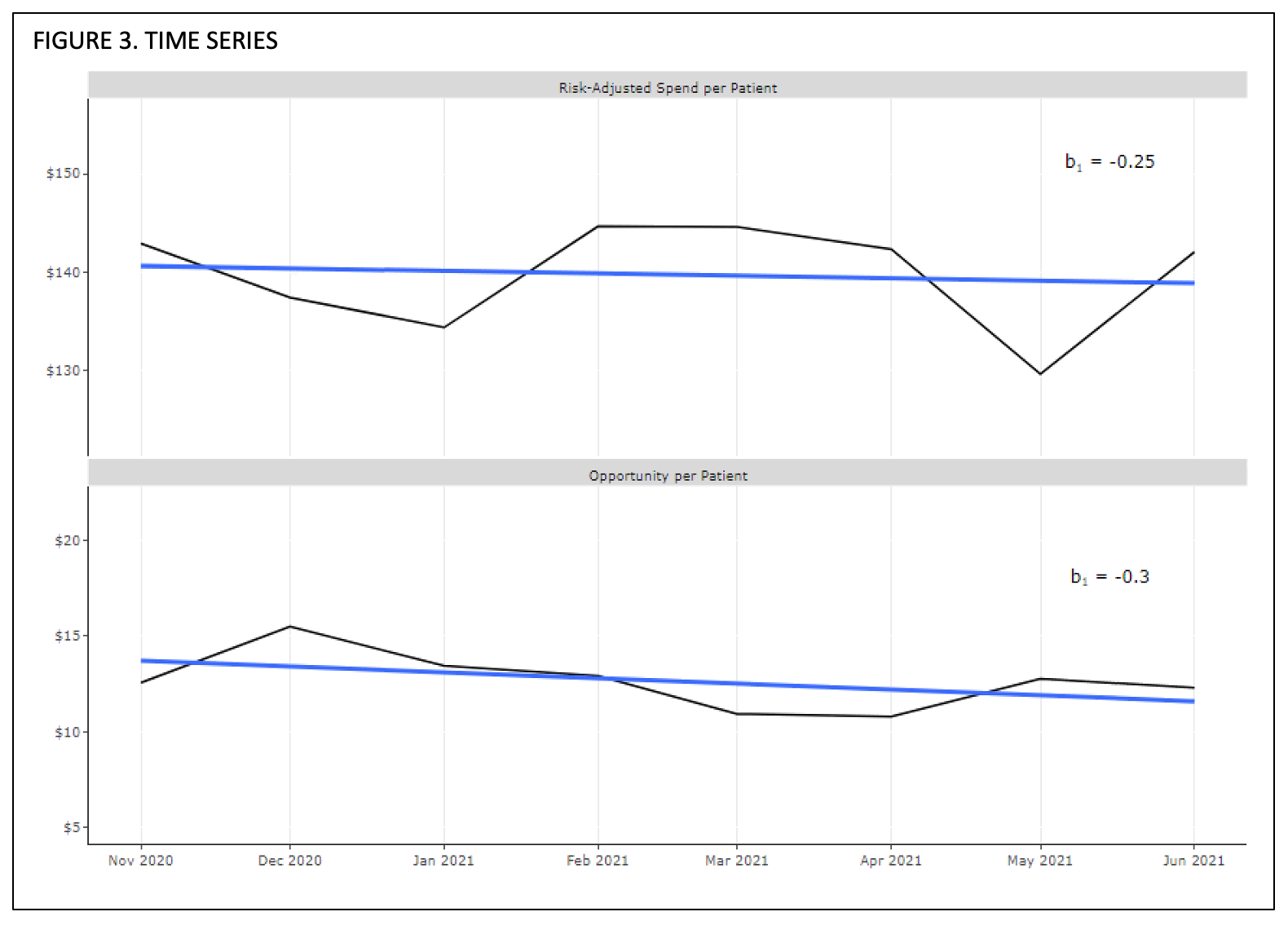
Discussion
Clinical stewardship reflects a mind-set that is difficult to create and even more difficult to measure. While it may be obvious that providers who spend more per admission have more opportunities to save money, the opportunities to reduce cost are not readily known at the point-of-care. IllumiCare has over 1400 clinical financial decision support opportunities in the medication and laboratory space that are markers of opportunities to make less costly decisions without compromising quality in the right clinical context. These opportunities predict 47% of the financial variation, risk-adjusted, in medication and laboratory spend in a patient’s admission.
Interestingly, the ceiling for savings is greater than the sum total of the opportunities attributed to the provider per patient. This implies a flywheel effect where an interested and attentive clinician-steward begins to ponder other opportunities to save that are not directly “nudged.” For example, IllumiCare may not nudge an expensive drug as an opportunity because there may be no alternative medication available. Astute clinicians can use the IllumiCare platform to notice expensive medications on the med list – these medications are purposely shown at the top of the med review screen. We consider such clinicians “advanced stewards” when they order these drugs less often on future admissions. This analysis shows that for every 1 dollar of decrease in average opportunities per provider per patient, the clinician actually saves up to 1.5 times that amount per admission. This reflects the activation of the stewardship program and its maximal effect being greater than the sum of the opportunities. This is a significant development in the stewardship program.
Finally, we analyzed length of stay, which remained fairly constant over the period of analysis. Thus, a decline in length of stay would not explain declining costs or opportunities per admission. We also examined whether clinicians who acted on opportunities and reduced their costs were merely shifting them to other providers. The study showed that was not the case, and these savings constituted a net reduction in the total cost of care.
Conclusion
This novel study strongly suggests that IllumiCare has a proprietary set of clinical financial decision support rules that are markers of opportunities to reduce financial variation in clinical care. The greater the “opportunity dollar amount” attributed to a provider, the greater the variation in care attributed to this provider. Indeed, when the provider focuses on these opportunities, cost of care and financial variation decline. Interestingly, the decline in overall spend per admission is steeper than the decline in dollar opportunity per provider per patient. This implies that these clinicians are on a path to stewardship and can transcend to savings beyond the sum total of these opportunities. We label these providers “advanced stewards” as they seek opportunities beyond “nudges” sent to them to reduce the cost of care while maintaining the quality of the care they deliver. There was no increase in risk adjusted morbidity and mortality in this study period.
About IllumiCare
Founded in 2014 in Birmingham, Ala. by a visionary physician and team of hospital IT experts, IllumiCare is dedicated to helping clinicians become better stewards of system and patient resources. Its Smart Ribbon® platform brings clinicians critical, patient-specific data in a focused view for expedited clinical decision making at the point of care, without disrupting clinical workflow.
iM. A. Morid, K. Kawamoto, T. Ault, J. Dorius and S. Abdelrahman, “Supervised Learning Methods for Predicting Healthcare Costs: Systematic Literature Review and Empirical Evaluation,” AMIA ... Annual Symposium proceedings. AMIA Symposium, 2017, pp. 1312-1321, 2018.
iiA. N. Leep Hunderfund, L. N. Dyrbye, S. R. Starr, J. Mandrekar, J. C. Tilburt, P. George, E. G. Baxley, J. D. Gonzalo, C. Moriates, S. D. Goold, P. A. Carney, B. M. Miller and S. J. Grethlein, “Attitudes toward cost-conscious care among U.S. physicians and medical students: analysis of national crosssectional survey data by age and stage of training,” BMC Medical Education, vol. 18, no. 275, 2018.
iiiAMA Council on Ethical and Judicial Affairs, “AMA Code of Medical Ethics’ Opinion on Physician Stewardship,” [Online]. Available: https://journalofethics.ama-assn.org/article/ama-code-medical-ethics-opinion-physician-stewardship/2015-11.
ivTsugawa Y, Jha AK, Newhouse JP, Zaslavsky AM, Jena AB. Variation in Physician Spending and Association With Patient Outcomes. JAMA Intern Med. 2017;177(5):675–682. doi:10.1001/jamainternmed.2017.0059.
vTsugawa, p. 677-678
viH.-Y. Kim, “Statistical notes for clinical researchers: simple linear regression 2 – evaluation of regression line,” Restorative dentistry & endodontics, vol. 43(3), no. e34, 2018.
viiT. Chai and R. R. Draxler, “Root mean square error (RMSE) or mean absolute error (MAE)? – Arguments against avoiding RMSE in the literature,” Geoscientific Model Development, vol. 7, pp. 1247-1250, 2014.
viiiA. de Myttenaere, B. Golden, B. Le Grand and F. Rossi, “Mean Absolute Percentage Error for regression models,” Neurocomputing, vol. 192, no. Advances in artificial neural networks, machine learning and computational intelligence Selected papers from the 23rd European Symposium on Artificial Neural Networks (ESANN 2015), pp. 38-48, 2016.
ixR. Williams, “Heteroskedacity,” 10 January 2020. [Online]. Available: https://www3.nd.edu/~rwilliam/stats2/l25.pdf [Accessed July 2021].
xB. Kim, “Understanding Diagnostic Plots for Linear Regression Analysis,” University of Virgina Library, 2015; A. Chouldechova, “Regression diagnostic plots,” [Online]. Available: https://www.andrew.cmu.edu/user/achoulde/94842/homework/regression_diagnostics.html [Accessed August 2021].
xiChouldechova
xiiChouldechova
xiiiKim

Study Reveals Access to Real-Time Alternatives Improve Cost Stewardship by 150%
- posted December 2021

A look at patients positive for COVID-19 & affects on cost and care.
– posted March 4, 2021


“One key element to the success of the THA Smart Ribbon is the fact that it is EMR agnostic. It does not directly integrate or interact with the EMR."
-posted May 25, 2021